Setup and Run Models
This section shows how to create new settings (either from scratch or
from existing settings) and run simulations with Model
instances, using the xarray extension provided by xarray-simlab. We’ll
use here the simple advection models that we have created in Section
Create and Modify Models.
The following imports are necessary for the examples below.
In [1]: import numpy as np

In [2]: import xsimlab as xs

In [3]: import matplotlib.pyplot as plt
Note
When the xsimlab package is imported, it registers a new
namespace named xsimlab for xarray.Dataset objects. As
shown below, this namespace is used to access all xarray-simlab
methods that can be applied to those objects.
Create a new setup from scratch
In this example we use the advect_model Model instance:
In [4]: advect_model
Out[4]:
<xsimlab.Model (4 processes, 5 inputs)>
grid
    spacing     [in] uniform spacing
    length      [in] total length
init
    loc         [in] location of initial pulse
    scale       [in] scale of initial pulse
advect
    v           [in] () or ('x',) velocity
profile
The convenient create_setup() function can be used to
create a new setup in a very declarative way:
In [5]: in_ds = xs.create_setup(
   ...:     model=advect_model,
   ...:     clocks={
   ...:         'time': np.linspace(0., 1., 101),
   ...:         'otime': [0, 0.5, 1]
   ...:     },
   ...:     main_clock='time',
   ...:     input_vars={
   ...:         'grid': {'length': 1.5, 'spacing': 0.01},
   ...:         'init': {'loc': 0.3, 'scale': 0.1},
   ...:         'advect__v': 1.
   ...:     },
   ...:     output_vars={
   ...:         'profile__u': 'otime'
   ...:     }
   ...: )
   ...:
Note
See below how the code cell here above can be automatically generated using
the %create_setup magic command.
A setup consists in:
one or more time dimensions (“clocks”) and their given coordinate values ;
one of these time dimensions, defined as main clock, which will be used to define the simulation time steps (the other time dimensions usually serve to take snapshots during a simulation on a different but synchronized clock) ;
values given for input variables ;
one or more variables for which we want to take snapshots on given clocks (time dimension) or just once at the end of the simulation (
None).
In the example above, we set time as the main clock dimension
and otime as another dimension for taking snapshots of \(u\)
along the grid at three given times of the simulation (beginning,
middle and end).
create_setup returns all these settings packaged into a
xarray.Dataset :
In [6]: in_ds
Out[6]:
<xarray.Dataset>
Dimensions:        (otime: 3, time: 101)
Coordinates:
  * time           (time) float64 0.0 0.01 0.02 0.03 0.04 ... 0.97 0.98 0.99 1.0
  * otime          (otime) float64 0.0 0.5 1.0
Data variables:
    grid__length   float64 1.5
    grid__spacing  float64 0.01
    init__loc      float64 0.3
    init__scale    float64 0.1
    advect__v      float64 1.0
If defined in the model, variable metadata such as description are also added in the dataset as attributes of the corresponding data variables, e.g.,
In [7]: in_ds.advect__v
Out[7]:
<xarray.DataArray 'advect__v' ()>
array(1.)
Attributes:
    description:  velocity
IPython (Jupyter) magic commands
Writing a new setup from scratch may be tedious, especially for big models with
a lot of input variables. If you are using IPython (Jupyter), xarray-simlab
provides helper commands that are available after loading the
xsimlab.ipython extension, i.e.,
In [8]: %load_ext xsimlab.ipython
The %create_setup magic command auto-generates the
create_setup() code cell above from a given model, e.g.,
In [9]: %create_setup advect_model --default --verbose
The --default and --verbose options respectively add default values found
for input variables in the model and input variable description as line comments.
Full command help:
In [10]: %create_setup?
Docstring:
::

  %create_setup [-s] [-d] [-v] [-n] model

Pre-fill the current cell with a new simulation setup.

positional arguments:
  model               xsimlab.Model object

optional arguments:
  -s, --skip-default  Don't add input variables that have default values
  -d, --default       Add input variables default values, if any (ignored if
                      --skip-default)
  -v, --verbose       Increase verbosity (i.e., add more input variables info
                      as comments)
  -n, --nested        Group input variables by process
File:      ~/checkouts/readthedocs.org/user_builds/xarray-simlab/conda/latest/lib/python3.7/site-packages/xsimlab/ipython.py
Run a simulation
A new simulation is run by simply calling the xsimlab.run()
method from the input dataset created above. It returns a new dataset:
In [11]: out_ds = in_ds.xsimlab.run(model=advect_model)
The returned dataset contains all the variables of the input
dataset. It also contains simulation outputs as new or updated data
variables, e.g., profile__u in this example:
In [12]: out_ds
Out[12]:
<xarray.Dataset>
Dimensions:        (otime: 3, time: 101, x: 150)
Coordinates:
  * otime          (otime) float64 0.0 0.5 1.0
  * time           (time) float64 0.0 0.01 0.02 0.03 0.04 ... 0.97 0.98 0.99 1.0
  * x              (x) float64 0.0 0.01 0.02 0.03 0.04 ... 1.46 1.47 1.48 1.49
Data variables:
    advect__v      float64 1.0
    grid__length   float64 1.5
    grid__spacing  float64 0.01
    init__loc      float64 0.3
    init__scale    float64 0.1
    profile__u     (otime, x) float64 0.0001234 0.0002226 ... 0.03916 0.02705
Note also the x coordinate present in this output dataset. x is declared
in advect_model.grid as an index variable and therefore has been
automatically added as a coordinate in the dataset.
Post-processing and plotting
A great advantage of using xarray Datasets is that it is straightforward to
include the simulation as part of a processing pipeline, i.e., by chaining
xsimlab.run() with other methods that can also be applied on Dataset (or
DataArray) objects.
For example, we can extract the values of profile__u at a given position on
the grid (and clearly notice the advection of the pulse):
In [13]: out_ds.profile__u.sel(x=0.75)
Out[13]:
<xarray.DataArray 'profile__u' (otime: 3)>
array([1.60522806e-09, 7.78800783e-01, 6.38150345e-40])
Coordinates:
  * otime    (otime) float64 0.0 0.5 1.0
    x        float64 0.75
Attributes:
    description:  quantity u
    units:        m
Or plot the whole profile for all snapshots:
In [14]: out_ds.profile__u.plot(col='otime', figsize=(9, 3));
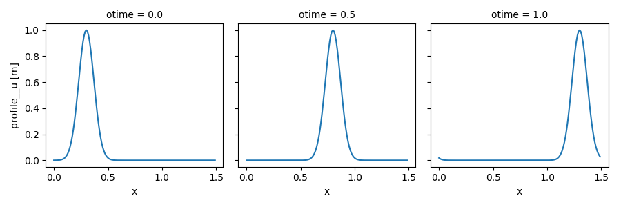
There is a huge number of features available for selecting data, computation, plotting, I/O, and more, see xarray’s documentation!
Reuse existing settings
Update inputs
In the following example, we set and run another simulation in which
we decrease the advection velocity down to 0.5. Instead of creating a
new setup from scratch, we can reuse the one created previously and
update only the value of velocity, thanks to
xsimlab.update_vars().
In [15]: in_vars = {('advect', 'v'): 0.5}

In [16]: with advect_model:
   ....:     out_ds2 = (in_ds.xsimlab.update_vars(input_vars=in_vars)
   ....:                     .xsimlab.run())
   ....:
Note
For convenience, a Model instance may be used in a context instead of providing it repeatedly as an argument of xarray-simlab’s functions or methods in which it is required.
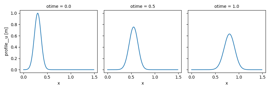
We plot the results to compare this simulation with the previous one (note the numerical dissipation as a side-effect of the Lax scheme, which is more visible here):
In [17]: out_ds2.profile__u.plot(col='otime', figsize=(9, 3));
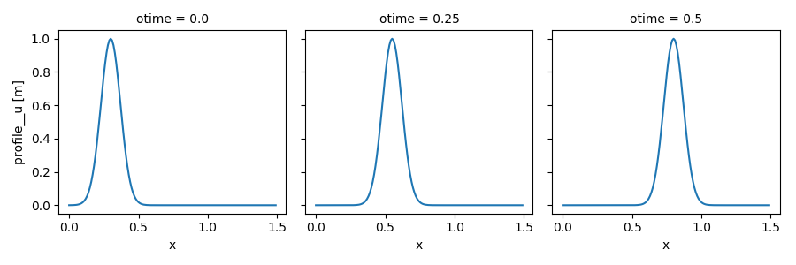
Update time dimensions
xsimlab.update_clocks() allows to only update the time
dimensions and/or their coordinates. Here below we set other values
for the otime coordinate (which serves to take snapshots of
\(u\)):
In [18]: clocks = {'otime': [0, 0.25, 0.5]}

In [19]: with advect_model:
   ....:     out_ds3 = (in_ds.xsimlab.update_clocks(clocks=clocks,
   ....:                                            main_clock='time')
   ....:                     .xsimlab.run())
   ....:

In [20]: out_ds3.profile__u.plot(col='otime', figsize=(9, 3));
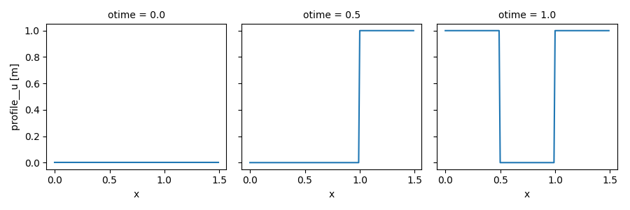
Use an alternative model
A model and its alternative versions often keep inputs in common. It
this case too, it would make sense to create an input dataset from an
existing dataset, e.g., by dropping data variables that are irrelevant
(see xsimlab.filter_vars()) and by adding data variables for
inputs that are present only in the alternative model.
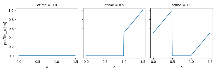
Here is an example of simulation using advect_model_src (source point and
flat initial profile for \(u\)) instead of advect_model :
In [21]: in_vars = {'source': {'loc': 1., 'flux': 100.}}

In [22]: with advect_model_src:
   ....:     out_ds4 = (in_ds.xsimlab.filter_vars()
   ....:                     .xsimlab.update_vars(input_vars=in_vars)
   ....:                     .xsimlab.run())
   ....:

In [23]: out_ds4.profile__u.plot(col='otime', figsize=(9, 3));
Time-varying input values
Except for static variables, all model inputs accept arrays which have a dimension that corresponds to the main clock. This is useful for adding external forcing.
The example below is based on the last example above, but instead of being fixed, the flux of \(u\) at the source point decreases over time at a fixed rate:
In [24]: flux = 100. - 100. * in_ds.time

In [25]: in_vars = {'source': {'loc': 1., 'flux': flux}}

In [26]: with advect_model_src:
   ....:     out_ds5 = (in_ds.xsimlab.filter_vars()
   ....:                     .xsimlab.update_vars(input_vars=in_vars)
   ....:                     .xsimlab.run())
   ....:

In [27]: out_ds5.profile__u.plot(col='otime', figsize=(9, 3));
Run multiple simulations
Besides a time dimension, model inputs may also accept another extra dimension that is used to run batches of simulations. This is very convenient for sensitivity analyses: the inputs and results from all simulations are neatly combined into one xarray Dataset object. Another advantage is that those simulations can be run in parallel easily, see Section Multi-models parallelism.
Note
Because of the limitations of the xarray data model, model inputs with a “batch” dimension may not work well if these directly or indirectly affect the shape of other variables defined in the model (e.g., grid size).
As a simple example, let’s update the setup for the advection model and set different values for velocity:
In [28]: in_ds_vel = in_ds.xsimlab.update_vars(
   ....:     model=advect_model,
   ....:     input_vars={'advect__v': ('batch', [1.0, 0.5, 0.2])}
   ....: )
   ....:
Those values are defined along a dimension named “batch”, that we need to
explicitly pass to xarray.Dataset.xsimlab.run() via its batch_dim
parameter in order to run one simulation for each value of velocity:
In [29]: out_ds_vel = in_ds_vel.xsimlab.run(model=advect_model, batch_dim='batch')

In [30]: out_ds_vel
Out[30]:
<xarray.Dataset>
Dimensions:        (batch: 3, otime: 3, time: 101, x: 150)
Coordinates:
  * otime          (otime) float64 0.0 0.5 1.0
  * time           (time) float64 0.0 0.01 0.02 0.03 0.04 ... 0.97 0.98 0.99 1.0
  * x              (x) float64 0.0 0.01 0.02 0.03 0.04 ... 1.46 1.47 1.48 1.49
Dimensions without coordinates: batch
Data variables:
    advect__v      (batch) float64 1.0 0.5 0.2
    grid__length   float64 1.5
    grid__spacing  float64 0.01
    init__loc      float64 0.3
    init__scale    float64 0.1
    profile__u     (batch, otime, x) float64 0.0001234 0.0002226 ... 9.064e-05
Note the additional batch dimension in the resulting dataset for the
profile__u variable.
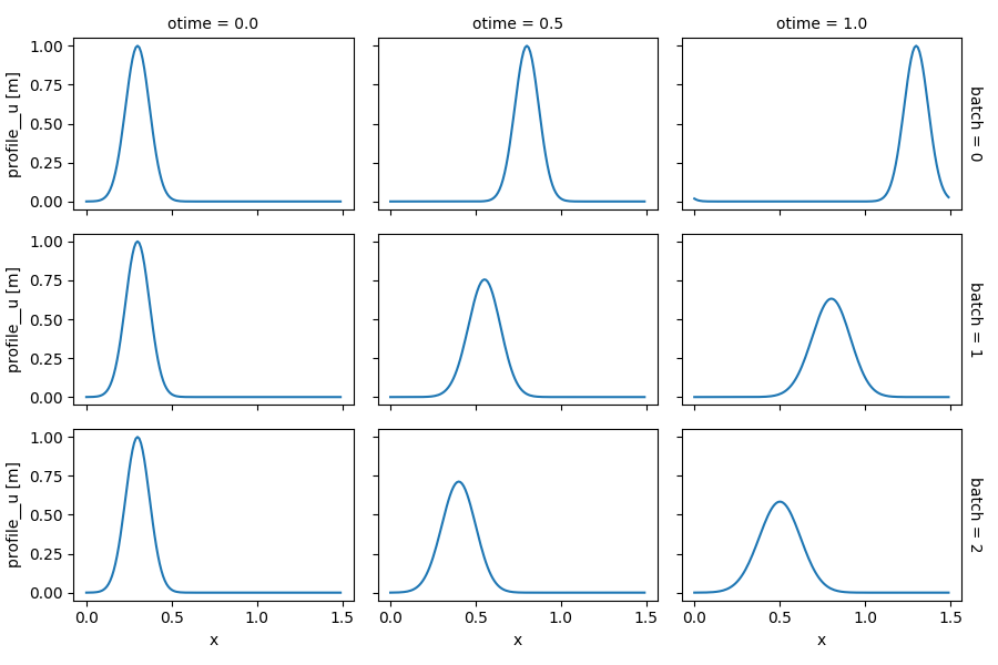
Having all simulations results in a single Dataset allows to fully leverage xarray’s powerful capabilities for analysis and plotting those results. For example, the one-liner expression below plots the profile of all snapshots (columns) from all simulations (rows):
In [31]: out_ds_vel.profile__u.plot(row='batch', col='otime', figsize=(9, 6));
Advanced examples
Running batches of simulations works well with time-varying input values, since the time and batch dimensions are orthogonal.
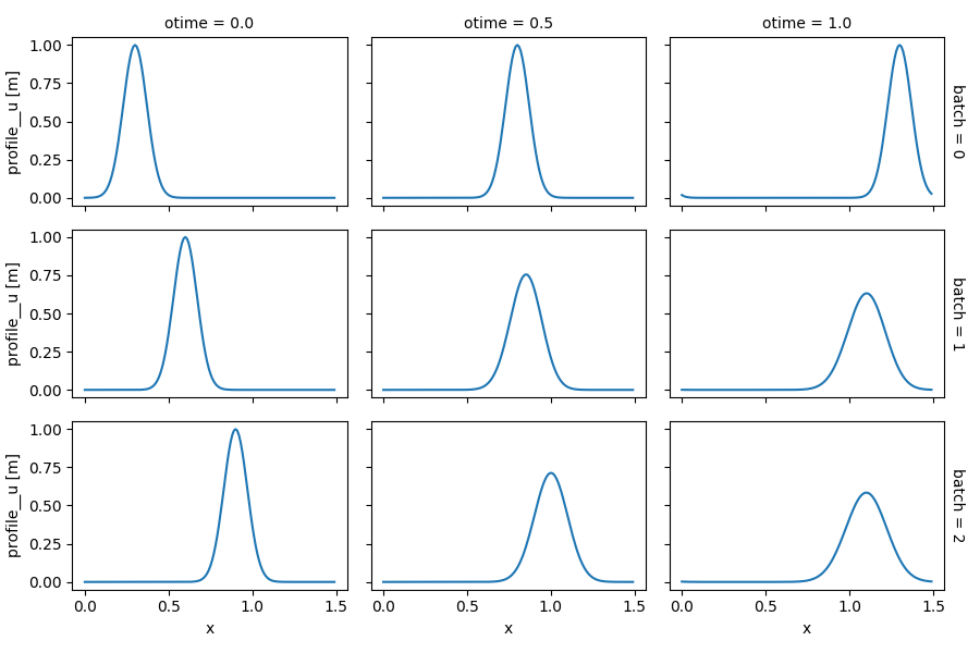
It is also possible to run multiple simulations by varying the value of several model inputs, e.g., with different value combinations for the advection velocity and the initial location of the pulse:
In [32]: in_ds_comb = in_ds.xsimlab.update_vars(
   ....:     model=advect_model,
   ....:     input_vars={'init__loc': ('batch', [0.3, 0.6, 0.9]),
   ....:                 'advect__v': ('batch', [1.0, 0.5, 0.2])}
   ....: )
   ....:

In [33]: out_ds_comb = in_ds_comb.xsimlab.run(model=advect_model, batch_dim='batch')

In [34]: out_ds_comb.profile__u.plot(row='batch', col='otime', figsize=(9, 6));
Using xarray.Dataset.stack() and xarray.Dataset.unstack()
respectively before and after run, it is straightforward to regularly sample
a n-dimensional parameter space (i.e., from combinations obtained by the cartesian
product of values along each parameter dimension). Note the dimensions of
profile__u in the example below, which include the parameter space:
In [35]: in_vars = {'init__loc': ('init__loc', [0.3, 0.6, 0.9]),
   ....:            'advect__v': ('advect__v', [1.0, 0.5, 0.2])}
   ....:

In [36]: with advect_model:
   ....:     out_ds_nparams = (
   ....:         in_ds
   ....:         .xsimlab.update_vars(input_vars=in_vars)
   ....:         .stack(batch=['init__loc', 'advect__v'])
   ....:         .xsimlab.run(batch_dim='batch')
   ....:         .unstack('batch')
   ....:     )
   ....:

In [37]: out_ds_nparams
Out[37]:
<xarray.Dataset>
Dimensions:        (advect__v: 3, init__loc: 3, otime: 3, time: 101, x: 150)
Coordinates:
  * otime          (otime) float64 0.0 0.5 1.0
  * time           (time) float64 0.0 0.01 0.02 0.03 0.04 ... 0.97 0.98 0.99 1.0
  * x              (x) float64 0.0 0.01 0.02 0.03 0.04 ... 1.46 1.47 1.48 1.49
  * init__loc      (init__loc) float64 0.3 0.6 0.9
  * advect__v      (advect__v) float64 0.2 0.5 1.0
Data variables:
    grid__length   float64 1.5
    grid__spacing  float64 0.01
    init__scale    float64 0.1
    profile__u     (otime, x, init__loc, advect__v) float64 0.0001234 ... 5.0...